Analyzing Dipole Moments in Molecular Dynamics Simulations

Molecular Dynamics is the study of the movement of atoms and observing how they move in space. From here you can infer something or reasons why some science behaves the way it does.

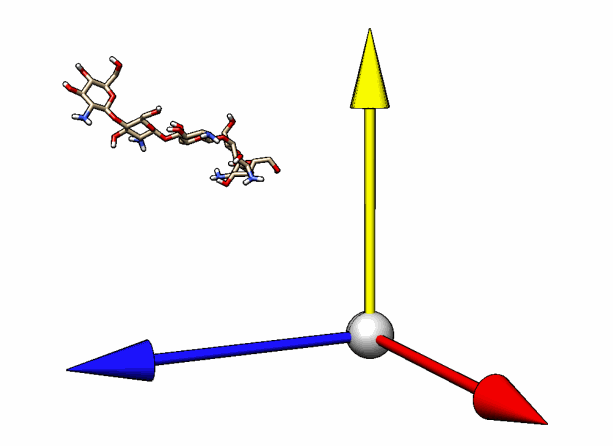
Positions of the atoms are one thing, but what about the charge? How do we analyze it? We look at a metric called the Dipole Moment.

The dipole moment is the magnitude of an electrical force as a distance between two point charges becomes greater or smaller.

Think of the each red dot as two different atoms perhaps Oxygen and Hydrogen. Oxygen is more electronegative and causes it’s area, a cloud if you will, around the nuclei to have a “negative” charge value.

The distance vector is from the negative to the positive side when you times that by the point charge value we achieve what we call a dipole moment.

dipole_moment = point_charge * distance

So what does this tell us?

The value of the dipole moment can change with respect to the chemical environment and attributes to binding and movement. Understanding the strength of these effects is of great importance to the molecular dynamics community because they can make better predictions. So let’s say you are running a simulation how do you analyze your dipole moment?

I don’t have access to my old simulations so take this next code with a grain of salt. We will be using MDAnalysis and Plotly to perform the data analysis and visualization to help us infer some things.

import MDAnalysis as mda
topology = os.path.join(current_directory, 'topology.psf')
trajectory = os.path.join(current_directory, 'trajectory.xtc')
universe = mda.Universe(topology, trajectory)

Note: So when loading the topology remember that it needs to have charge information, psf file for me contains that information but if you just have the initial reference frame it won’t work.

Set up our analysis frames:

starting_frame = 0
ending_frame = 50000
skip = 10
data = universe.trajectory[starting_frame:ending_frame:skip]
atom_group = universe.select_atoms('segid CHAIN_ID')

We will have to take each atom in the system and sum each individual dipole vector to get the overall dipole vector of the system.

for timestep in data:
  total_dipole_vectors = []
  for atom in atom_group: 
                    
     dipole_vector = [
         atom.position[0] * atom.charge, # X
         atom.position[1] * atom.charge, # Y
         atom.position[2] * atom.charge  # Z
     ]         
     total_dipole_vectors.append(dipole_vector)

Once we have that we can take the vector with respect to something to get an idea as to how much that vector moves around.

The green arrow indicates the dipole vector and for my simulation and I was applying an electrical field in some direction with a vector. So I wanted to see how the electrical field applied in the X direction influenced the dipole moment of my system. To add vectors just add the items in the list.

dipole_angles = []
from numpy import rad2deg
for timestep in data:
    total_dipole_vectors = []
    for atom in atom_group: 
                    
       dipole_vector = [
             atom.position[0] * atom.charge, # X
             atom.position[1] * atom.charge, # Y
             atom.position[2] * atom.charge  # Z
       ]
       total_dipole_vectors.append(dipole_vector)
       angle = rad2deg(
             mda.lib.mdamath.angle(
               add_vectors(total_dipole_vectors), [1, 0 ,0]
             )
       )
       
       dipole_angles.append(angle)

Plot the distribution:

# Distribution Plot of the Dipole Vector vs the Electric Field Vector
import plotly.figure_factory as ff 
colors = ["#A800FF", "#0079FF", "#00F11D", "#FF7F00", "#FF0900"] 
bin_size = .5
bin_width = ''
group_labels = [         
        'High',       
        'Mid',       
        'Low',      
        'No Field',           
 ]  
# Create distplot with custom bin_size 
fig = ff.create_distplot(
       [ 
         dipole_angles,
         # dipole_electric_field_high_angles,
         # dipole_electric_field_mid_angles,
         # dipole_electric_field_low_angles,
       ], 
     group_labels, 
     bin_size=bin_size, 
     show_hist=False,
     show_rug=False, 
     colors=colors
)  
fig.update_layout(legend=dict(itemsizing='constant')) fig.update_layout(
    legend=dict(    
        orientation="h",      
        yanchor="bottom",      
        y=1.02,     
        xanchor="right",      
        x=1.2,           
        font = dict(family = "Arial", size = 45),         
        bordercolor="LightSteelBlue",  
        borderwidth=2,     
    ),   
   legend_title = dict(
        font = dict(family = "Arial", size = 45))
    ) 
fig.update_traces(line=dict(width=10))  
fig.update_xaxes(    
      ticks="outside", 
      tickwidth=3,    
      tickcolor='black',                      
      tickfont=dict(family='Arial', color='black', size=50),                  
      title_font=dict(size=46, family='Arial'),                  
      title_text='Angle (θ)',     
      ticklen=15,            
      range=[0, 95],       
      tickvals=[0,30, 60, 90, 120] 
) 
fig.update_yaxes(    
      ticks="outside",             
      tickwidth=3,              
      tickcolor='black',    
      title_text='Probability Density',                  
      tickfont=dict(family='Arial', color='black', size=50),                  
      title_font=dict(size=46, family='Arial'),                  
      ticklen=15,               
      tickvals=[0.012, 0.024] 
)     
fig.update_layout(   
      title_text="Dipole Vector wrt E-Field Distribution",         
      title_font=dict(size=40, family='Arial'),         
      template='simple_white',  
      xaxis_tickformat = 'i',   
      bargap=0.2,
      height=600,    
      width=1400 
)

By taking the probability distributions we can get an idea of the angle forming:

And check out what happens in the simulation: